Teaching a diffusion model physics

Jan-Paul Lerch · 20 October 2026

A diffusion model learns what its training data look like, but not why they look that way. Now, if the data are solutions of a physical equation, then every sample should satisfy this equation, too. Nothing in the standard training objective asks for this, though: the model reproduces the law only as far as it happens to pick it up from examples.

Bastek, Sun and Kochmann propose to write the law into the training directly, see Physics-Informed Diffusion Models (ICLR 2025). I worked through the paper for a talk in the seminar Mathematics of Machine Learning at TU Berlin earlier this year and reimplemented it on a small problem, to see how it behaves in practice. In the following we first motivate why one wants a generative model here at all, then look at where the physics enters, and finally at what happens on an example.

Why a generative model at all

Our running example is the Poisson equation on the unit square,

-\Delta u = f \quad \text{in } \Omega = [0,1]^2, \qquad u = 0 \text{ on } \partial\Omega,

which describes, for example, steady-state heat conduction: $f$ is a heat source and $u$ the resulting temperature. In practice the source is rarely known exactly. Material parameters, boundary data and source terms all carry uncertainty, and what we actually want is the distribution of possible solutions, not a single best guess.

A neural surrogate trained with a mean squared error cannot deliver this. Under small perturbations of its input it essentially returns the conditional mean, because this is what minimises the squared loss. So the variance, which is the interesting part, is averaged away. To recover it, the model has to generate samples instead of predicting a single one, and today this means a diffusion model.

Diffusion in one paragraph

A diffusion model is defined by a forward process which slowly destroys the data: Starting from a clean field $x_0$ , it adds Gaussian noise over $T$ steps, and every intermediate state has a closed form

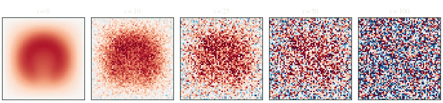
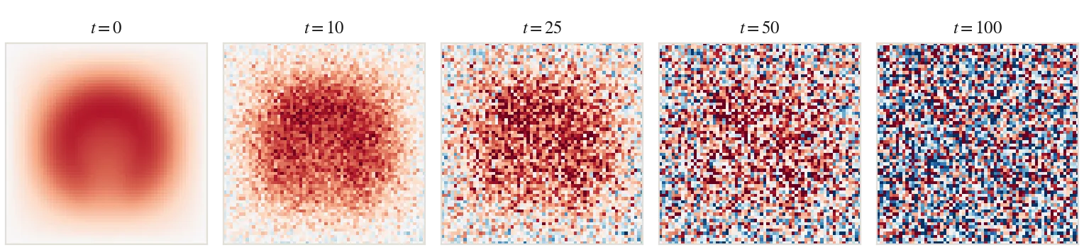
x_t = \sqrt{\bar\alpha_t}\, x_0 + \sqrt{1-\bar\alpha_t}\, \varepsilon, \qquad \varepsilon \sim \mathcal{N}(0, I).

Five panels showing a smooth temperature field turning into pure noise as the time step increases from 0 to 100. — The forward process on a solution of the Poisson equation, with a cosine noise schedule and T = 100. The model learns to run this backwards.

Then a neural network, the denoiser, is trained to look at a noisy $x_t$ and to estimate the clean field $\hat x_0(x_t, t)$ it came from. This single network is enough to run the process in reverse: Starting from pure noise and denoising step by step, we obtain a new sample from the data distribution. The idea goes back to Sohl-Dickstein et al. (2015), and the form used here to Ho, Jain and Abbeel (2020).

Where the physics goes

We write the PDE as a residual $\mathcal{R}(x) = -\Delta x - f$ , so that $x$ solves the equation if and only if $\mathcal{R}(x) = 0$ . A physics-informed neural network (PINN), see Raissi, Perdikaris and Karniadakis (2017), simply adds $\|\mathcal{R}\|^2$ to its loss. For a diffusion model this does not work directly, because during training the network only ever sees noisy fields $x_t$ , and noise destroys the structure of the PDE: Even if $x_0$ is an exact solution, $\mathcal{R}(x_t)$ is nowhere near zero.

The paper’s way out is to evaluate the residual not on $x_t$ , but on the denoiser’s own estimate $\hat x_0(x_t, t)$ , which the network computes anyway. Moreover, the physics term is weighted by the variance of the reverse process at step $t$ . Then the full training loss reads

\mathcal{L}_{\text{PIDM}} = \mathbb{E}\Big[\, \lambda_t \,\big\|x_0 - \hat x_0(x_t, t)\big\|^2 \;+\; \frac{1}{2\bar\Sigma_t}\, \big\|\mathcal{R}\big(\hat x_0(x_t, t)\big)\big\|^2 \Big].

The first term is the standard diffusion loss, the second term is the PDE residual. Now, the factor $1/(2\bar\Sigma_t)$ does the actual work: For small $t$ the estimate $\hat x_0$ is sharp and the physics is enforced strictly. For large $t$ the estimate is only a blurry average, and so the penalty relaxes. The only new hyperparameter is an overall strength $c$ inside $\bar\Sigma_t$ .

Two properties make this more than a heuristic. First, the residual term comes from a Gaussian likelihood of a “virtual observation” $\mathcal{R} = 0$ , and the paper shows that for data satisfying the PDE it does not move the optimum of the score matching objective. In other words, in the ideal case it cannot make the model worse, it only shapes how the training gets there. Second, the sampling is unchanged: There is no guidance, no projection and no extra cost at inference.

Certainly there is a catch for nonlinear equations. The residual of the averaged estimate is not the average of the residual, $\mathcal{R}(\mathbb{E}[x_0 \mid x_t]) \neq \mathbb{E}[\mathcal{R}(x_0) \mid x_t]$ , so at high noise levels the physics term is biased; this is the so-called Jensen gap, named after Jensen’s inequality. For a linear PDE like the Poisson equation this gap vanishes, which is one reason why it is a convenient test case.

Trying it on Poisson

To see the effect, I trained two otherwise identical models: a plain diffusion model and the physics-informed version. The training data were 2,000 pairs $(f, u)$ on a $64\times 64$ grid, where each source $f$ was a sum of three to eight random Gaussian bumps and $u$ came from a sparse solver. The network was a U-Net with about 4.5 million parameters, trained for 50,000 iterations, which took about half an hour on one A100.

The residual is pleasantly cheap to implement: The five-point stencil of the Laplacian is just a $3\times 3$ convolution with frozen weights, so PyTorch differentiates the physics loss by itself.

The interesting test is what happens outside the training distribution. Both models have only ever seen smooth Gaussian blobs. So I gave them sources with sharp edges and geometric structure: an interdigital capacitor, an L-shaped electrode and a charged plate with a hole.

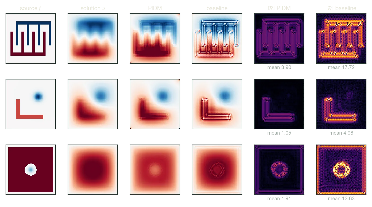
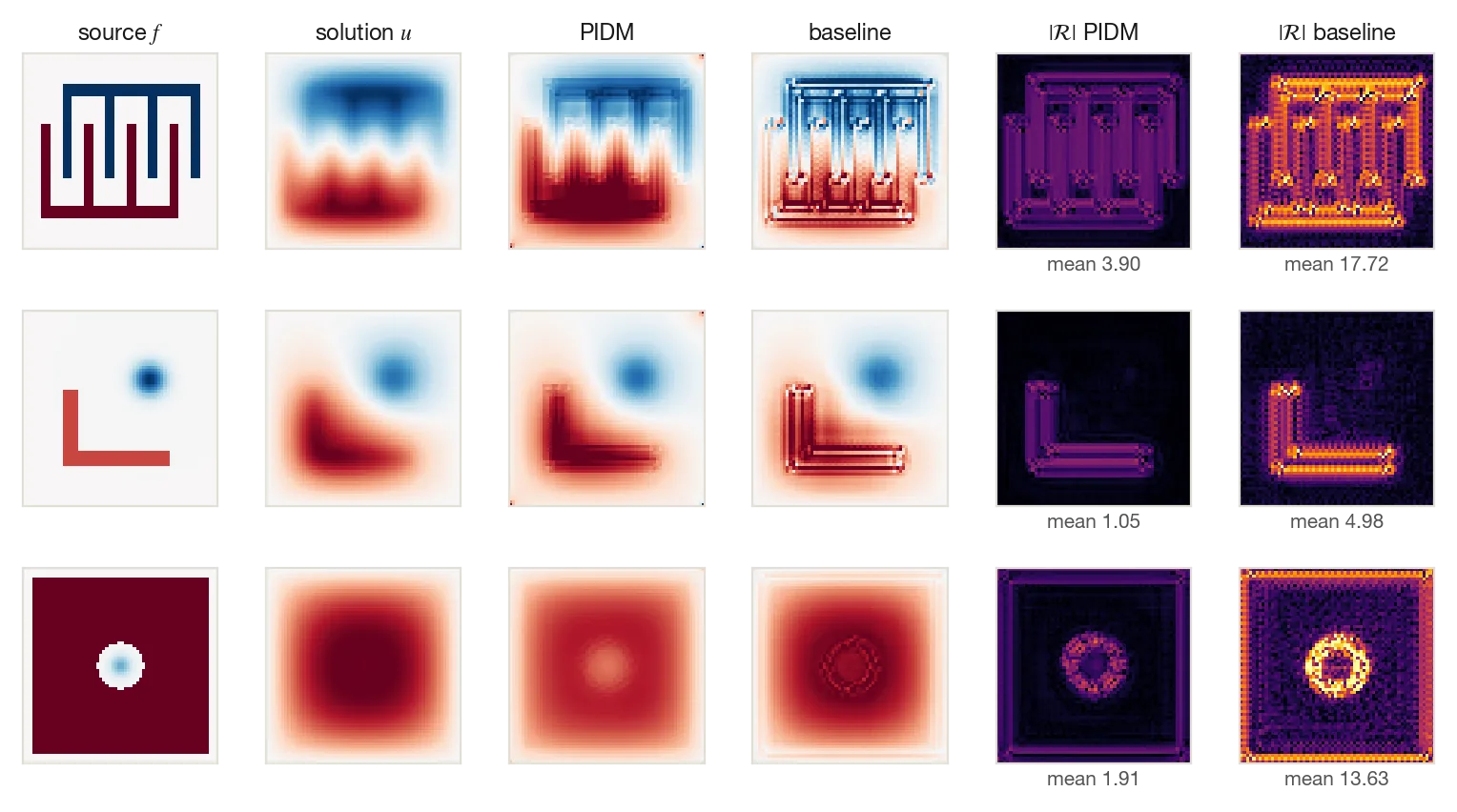
Comparison grid for three unseen source fields. Columns show the source, the true solution, the PIDM sample, the baseline sample, and the PDE residual of both models. The residual of PIDM is visibly darker in every row. — Out-of-distribution sources: an interdigital capacitor, an L-shaped electrode, and a charged plate with a hole. The right two columns show the pointwise residual |−Δu − f| on a shared scale, with its mean below each panel.

On every shape the residual of the physics-informed model is between 4.5 and 7 times lower. The baseline produces fields which look plausible, but violate the equation along every edge of the source. The samples of PIDM are visibly smoother there, because under the Laplacian a sharp artefact is expensive.

However, this needs two qualifications. On one hand, a lower residual is not the same as a more accurate solution. Measured by the mean squared error against the true $u$ , the picture is mixed: on some shapes PIDM is closer, on others the baseline is. The physics term makes the samples more consistent with the equation, but it cannot supply information about the solution which the training data lacked. On the other hand, PIDM is only as good as the residual it is given. My residual lives on the interior of the grid, and the four corner pixels never enter any stencil, so nothing constrains them. In the samples they drift freely. This is harmless here, but it is a good reminder that the model enforces exactly the physics we write down, and nothing more.

A medical reading

The Poisson equation also describes the simplest case of Darcy flow in tissue. If we read $f$ as a perfusion source and $u$ as the interstitial pressure, then we can ask the same model about kidney-like patterns: a cortex ring with the indent of the hilum, and arterial inflow at the hilum next to a draining vein.

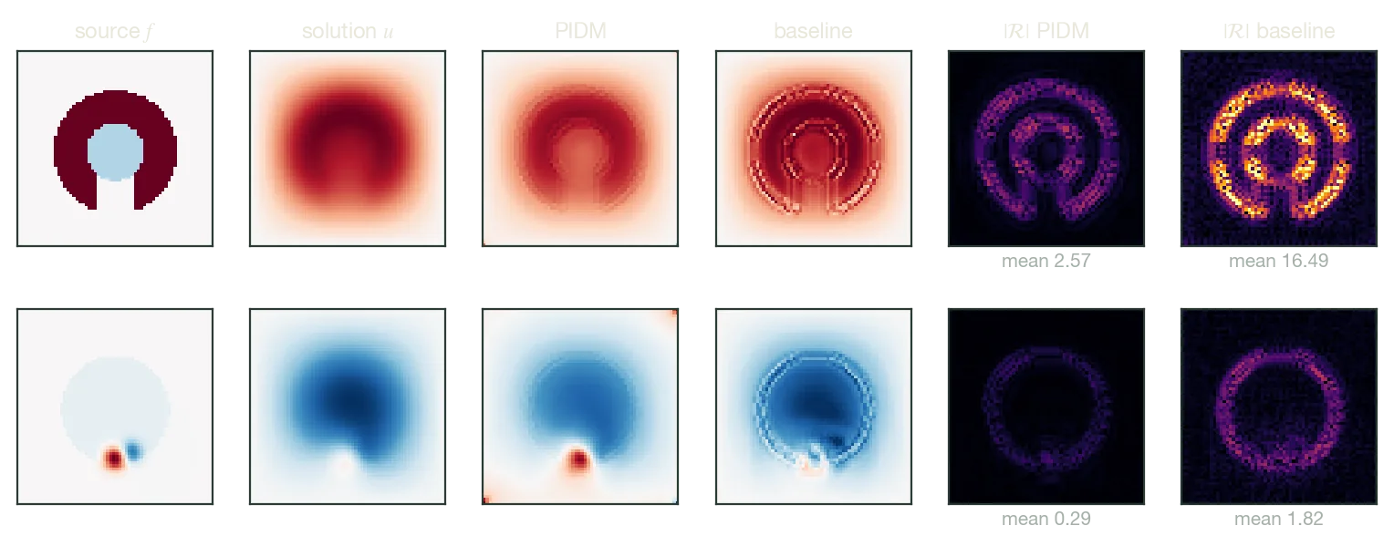
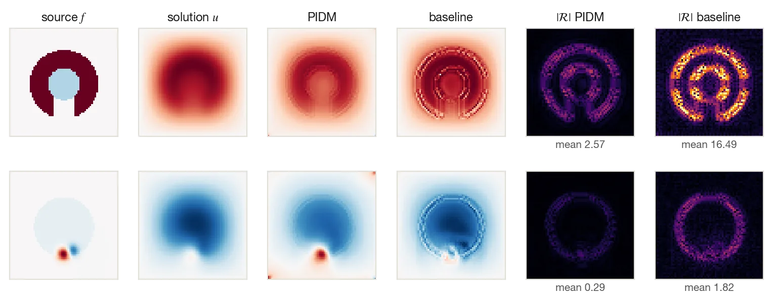
Comparison grid for two kidney-inspired source patterns, laid out like the previous figure. The residual of PIDM is again much smaller than that of the baseline. — Kidney-inspired perfusion sources: cortex ring and hilum inflow. Neither shape appears in the training data.

Again, the residual drops by a factor of about six in both cases. Of course this is a toy: Real tissue has varying permeability, the domain is not a square, and nobody should read clinical meaning into it. Nonetheless, it shows the appeal of the approach. A generative model which has learned the physics generalises far better to source geometries it has never seen than one which has only learned what typical solutions look like.

Physics at training time or at sampling time

DiffusionPDE takes the opposite route. It trains a plain diffusion model and enforces the PDE only during sampling, by nudging every denoising step along the gradient of the residual and of a loss on sparse observations. On one hand this makes it flexible: the equation can be exchanged without retraining, and it can solve inverse problems from a handful of measurements. On the other hand the sampler becomes more expensive. Conversely, PIDM bakes the physics into the weights and samples at the usual cost, but a new equation needs a new model.

So the two approaches are complementary, and an immediate follow-up question is whether they can be combined. A second question is how far the idea carries beyond linear problems, where the Jensen gap no longer vanishes. What remains in any case is how little the physics-informed version needs: one extra term in the loss, a weighting which follows from the probabilistic model instead of being tuned by hand, and a proof that this term cannot pull the model away from the data.